Why AP Confused Me in IR (And How I Finally Understood It)

Context #
I've been working on an image search system for a client, which retrieves most similar images from a database given a user's query image. I usually use top-$K$ accuracy metrics when prototyping image similarity apps, where I check if any relevant image appears in the top-$K$ recommendations or whether the query's class label is included in the unique top-$K$ categories of the retrieved result.
These metrics have been useful, but as the model’s performance improved on the current datasets, we found that top-$K$ accuracy had become a bit too lenient. So, we decided to include mean average precision (mAP) in the evaluation to gain a more nuanced understanding of the model’s retrieval performance.
I knew that the AP in object detection (OD) is defined as the area under the precision-recall curve (AUC-PR), but the definition of AP seemed a bit different in the context of information retrieval (IR). After doing some research, I realized that there’s a key difference: AP in IR approximates AUC-PR without interpolated precision, whereas AP in OD is explicitly defined as AUC-PR with interpolated precision. Additionally, retrieval and recommender systems are often evaluated with AP@K that has multiple variants, and it was painful to figure them all out.
The mathematical terms used in AP and AP@K definitions were also confusing because many online resources gloss over whether these terms are calculated based on the entire dataset or just the retrieved sequence. I found Evidently AI's article to be quite comprehensive, but this article on builtin.com is possibly the best resource as it clearly describes how AP is defined in both IR and OD contexts. While these posts already cover the topic well, I'd like to add a few nuances that really helped me understand these metrics better.
Situation #
We have an IR or some kind of search system (items can be anything like documents or images) that retrives $N$ most relevant items, given a user's query $q$ (e.g., a single image, a set of search keywords, etc.). We want to evaluate how good the returned results are for this particular query, and also know how well it performed for $M$ queries on average. The system is not perfect and items within this retrieved list can actually be "relevant" or "not relevant" for the user.
Here’s a quick visualization to clarify the key symbols used throughout this post: 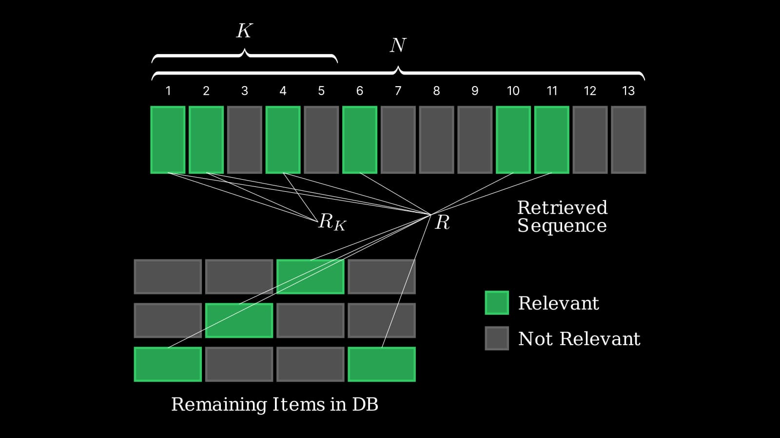
Notation:
- $N$: Total number of retrieved items
- $K$: Cut-off rank for top-$K$ evaluation (user-specified)
- $R$: Total number of relevant items in the dataset (for a given query)
- $R_K$: Number of relevant items within the top-$K$ retrieved results
In the above visualization, $K = 5$.
Precision and Recall in IR #
P vs P@K #
First, we need to understand AP because mAP is just an averaged value of APs. To do so, we start by understanding precision in IR. Precision in IR is similar to OD and the denominator is the total number of retrieved (predicted) items. $Precision@K$ or $\text{P@}k$ is just a precision at a fixed cutoff point ($K$). $K$ is user-specified (something you decide).
$$ \begin{aligned} \text{Precision@K} &= \frac{\text{Number of relevant items in top } K}{K} \\ &= \frac{R_K}{K} \end{aligned} $$
Recall vs recall@K #
I'd also like to mention these before explaining AP. They are basically just regular recalls but $Recall@K$ has a cutoff point (K) for calculating the numerator term. Note that the denominator is both the total number of relevant items in the entire dataset for a particular query.
$$ \begin{aligned} \text{Recall@K} &= \frac{\text{Number of relevant items in top } K}{R} \\ &= \frac{ R_K }{R} \end{aligned} $$
AP vs AP@K in IR #
This was the most confusing part for me. I'd like to describe two types of AP here:
- 📊 $AP$: Average Precision calculated over the retrieved ranked list for query $q$. The result is normalized over the total number of relevant items in the dataset ($R$) . It is alsmot equal to the AUC-PR without interpolated precisions.
- 🎯 $AP@K$: Average Precision that only considers top-$K$ recommendations for query $q$ in the retrieved sequence. The normalization factor depends on specific definitions.
I'll explain the standard AP first, and then AP@K.
Average Precision (AP) #
AP is sometimes denoted as $AP(q)$, but people just call it as "AP" because it's usually obvious that we compute AP for a single query in IR. Considering this, here is the definition that I find intuitive:
Where:
- $N$: Total number of items in the retrieved ranked list.
- In large-scale systems, this usually refers to the number of retrieved items.
- In small-scale systems (e.g., when computing a full similarity matrix), $N$ can be the size of entire dataset.
- $R$: Total number of relevant items in the dataset (for the current query)
- $\text{P@}k$: Precision at rank $k$
- $rel(k)$: Indicator function (1 if the item at rank $k$ is relevant, 0 otherwise)
Unlike precision, the denominator of AP is the actual total number of relevant items in the entire dataset $R$, not just the number of relevant items retrieved. For example, if there are 10,000 relevant items in your dataset for the query and your retrieval system returns 1,000 items, you iterate over those 1,000 items to compute AP. However, you still use 10,000 as $R$ in the denominator to reflect the fact that there are many relevant items the system might have missed.
Both precision and AP measure how accurate the predictions are in identifying relevant items, but AP goes a step further by considering the order of relevant items in the retrieved sequence, rewarding relevant items placed towards the top. This focus on ranking is crucial in IR, since users expect the most relevant results to appear at the top of the list. Precision only calculates the proportion of relevant items retrieved, and it does not account for their positions in the ranking. As a result, precision cannot evaluate how well a system prioritizes relevant items in higher ranks, which is often key to a good user experience.
Average Precision at K (AP@K) #
In practice, we often care more about the retrieval performance in the top-$K$ results rather than across the entire retrieved list. This is where AP@K comes in—it only evaluates the top-$K$ retrieved items, focusing on how well the system ranks relevant items at the top Interestingly, there are multiple variants for AP@K definitions. Here, I list two of the most common ones:
$$ AP_1@K = \frac{1}{R_K} \sum_{k=1}^{K} \text{P@}k \times rel(k) $$
$$ AP_2@K = \frac{1}{\min(K, R)} \sum_{k=1}^{K} \text{P@}k \times rel(k) $$
Where:
- $K$: Cut-off rank for top-$K$ evaluation (user-specified; i.e., top-10)
- $R_K$: Total number of relevant items within the top-$K$ retrieved results
- $R$: Total number of relevant items in the dataset (for the current query)
- $\text{P@}k$: Precision at rank $k$ (same as AP)
- $rel(k)$: Indicator function (1 if the item at rank $k$ is relevant, 0 otherwise) (same as AP)
For clarity, I'll refer to the first definition as $AP_1@K$ and the second one as $AP_2@K$.
Based on my research, $AP_2@K$ seems to be more commonly used, especially in research papers. I have seen a moderate number of online articles using $AP_1@K$, but in academic research, $AP_2@K$ appears to be more commonly used. For example, I found the following papers defining AP@K using the $AP_2@K$ formula:
- Deep Learning Based Dense Retrieval: A Comparative Study
- Collaborative Ranking with a Push at the Top
- Inquire: A Natural World Text-to-Image Retrieval Benchmark
The "INQUIRE" paper explains in more detail how different research works have defined AP@K. If you're curious, I recommend checking out Appendix G of that paper. Their explanation suggests that $AP_2@K$ originates from the TREC book (2005), but unfortunately I don’t have access to it.
Another example is the implementation of RetrievalMAP() in torchmetrics (source) using this definition. That said, there are also a number of sources that only mention the $AP_1@K$ definition, such as:
Ultimately, which AP@K definition to use is a user choice, and I'll describe the intuitions behind these below to help you decide.
$AP_1@K$ #
This definition of AP@K normalizes the sum of precision scores by $R_K$, which is the number of relevant items within the top-$K$ results. Intuitively, this version measures how precise the top-$K$ retrieval result was, as it’s just an average of Precision@K. If no relevant items are found in the top-$K$, $R_K = 0$, and AP@K is undefined (though often treated as zero in implementations).
However, the issue with this definition is that it’s a purely precision-oriented metric, and the system can cheat by placing only a few relevant items within the top-$K$. For example, if the system retrieves just a single relevant item at rank 1 and misses all other relevant items, AP@K is still 1.0. This makes it less strict compared to $AP_2@K$, which explicitly penalizes for missing relevant items outside the top-$K$.
$AP_2@K$ #
Unlike $AP_1@K$, this version penalizes missing relevant items if they were not retrieved within the top-$K$, since the denominator is $\min(K, R)$.
This means that it rewards the system for ranking more relevant items in the top-$K$, even if they're placed towards the bottom in that range. For example, consider a case where $R=2$ and the system retrieves this sequence: $$[1, 0, 0, 0, 0]$$
$AP_1@K = 1.0$, but $AP_2@K = 0.5$ since one relevant item is still missing.
Now, if the system promotes another relevant item into the top-5 like this: $$[1, 0, 0, 0, 1]$$
$AP_1@K = AP_2@K = 0.7$.
This ranking is more desirable than the previous one, but we can see that $AP_1@K$ decreases by doing so, while $AP_2@K$ properly rewards the improved ranking.
AP@K Examples #
To understand how these AP@K definitions behave more, let's consider these two examples:
Ex1: $AP_1@K$ and $AP_2@K$ are the same #
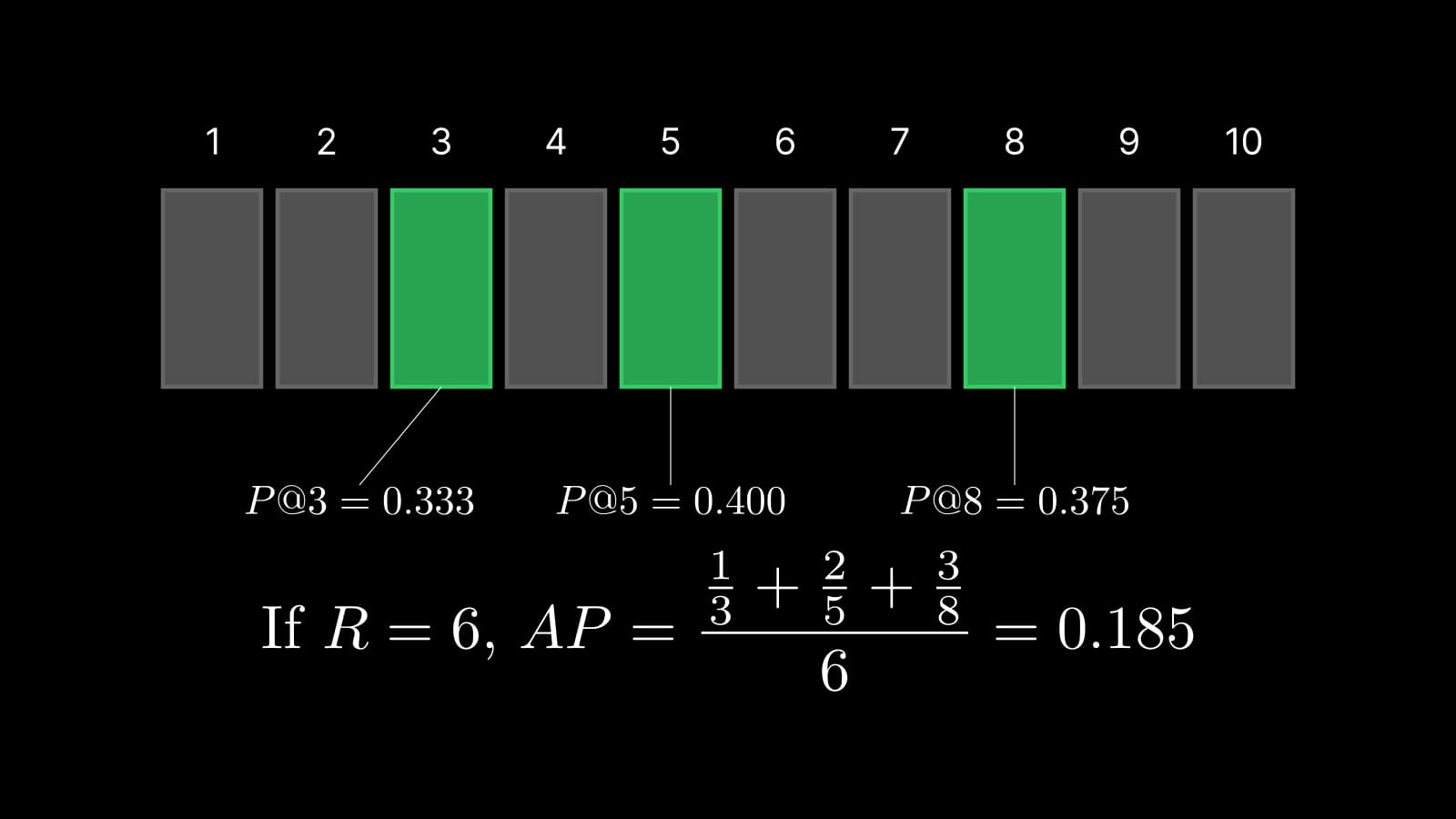
A system returns a sequence: $$[0, 0, 1, 0, 1, 0, 0, 1, 0, 0]$$ for your query (1 = relevant, 0 = not relevant) where the actual total number of relevant item is 3 (all relevant items retrieved). To build some intuition I made a simple animated example here:
As for the summation part, we simply compute a precision at each relevant item and take the average of those:
precision = TP / (TP + FP)
precision@3 = 1 / (1 + 2) = 0.333
precision@5 = 2 / (2 + 3)  = 0.4
precision@8 = 3 / (3 + 5) = 0.375
In this particular example, the relevant items were scattered across ranks and two of the items were ranked at 5 and 8 even though they're relevant, resulting in a rather lower AP@10 of 0.369.
This example shows that when all relevant items are retrieved within the top-$K$, $AP_1@K$ and $AP_2@K$ are identical.
Ex2: $AP_1@K$ is 1.0, $AP_2@K$ is low #
A system returns a sequence: $$[1, 1, 0, 0, 0, 0, 0, 0, 0, 0]$$ where the actual total number of relevant item is 6 (4 relevant items were missed).
$$ \begin{aligned} AP_1@K &= \frac{\frac{1}{1} + \frac{2}{2}}{2} = 1.0 \\ AP_2@K &= \frac{\frac{1}{1} + \frac{2}{2}}{6} = 0.333 \end{aligned} $$
Here, $AP_1@K$ is 1.0 because it rewards placing just a few relevant items toward the top, even though 4 relevant items were completely missed. If you are only interested in evaluating the precision-like aspect of system performance, this may be fine. However, $AP_2@K$ penalizes the system for failing to retrieve all relevant items and results in a much lower value.
In most recommender systems, we ideally want to fill the top ranks with as many relevant items as possible. For this example, an ideal ranking would look like this: $$[1, 1, 1, 1, 1, 1, 0, 0, 0, 0]$$
In this case, $AP_1@K$ does not distinguish between these two cases and remains 1.0, while $AP_2@K$ properly rewards this by achieving a perfect 1.0 score.
This highlights why $AP_2@K$ is often preferred in practice, as it better reflects real-world scenarios where we care about not just ranking precision, but also about missing relevant items (recall-like aspect).
mAP in IR #
The mean Average Precision (mAP) is simply the AP values averaged over multiple queries. If we have $M$ queries, each with its own AP, the formulae for mAP and mAP@K are:
$$ \text{mAP@K} = \frac{1}{M} \sum_{j=1}^{M} \text{AP@K}_j $$
Where:
- $M$ is the total number of queries,
- $\text{AP}_j$ is the Average Precision for the $j$-th query,
- $\text{AP@K}_j$ is the Average Precision at cutoff $K$ for the $j$-th query.
$M$ is just a user-specified parameter, so for example you can compute mAP for all the query items in your test set or per-category mAPs depending on your dataset.
Relation to PR Curve #
Precision-Recall Curve #
AP (not AP@K) in IR is almost equal to AUC-PR without interpolated precision because it’s calculated as a sum of precisions at every relevant item. The actual AUC-PR may differ slightly since it's defined as the continuous integration over the entire precision-recall curve.
In contrast, AP in OD is explicitly defined as the AUC-PR with interpolated precision, where the PR curve is smoothed to be non-decreasing. This interpolation stabilizes the evaluation, making AP in OD exactly equal to the area under the interpolated PR curve.
Here, I provide an example of how you can compute the points to plot a PR curve using the same example I used earlier. You need pairs of (Precision@K, Recall) points at every rank:
| Rank | Rel | Precision@K | Recall |
|---|---|---|---|
| 1 | 0 | — | 0/3 (0.00) |
| 2 | 0 | — | 0/3 (0.00) |
| 3 | 1 | 1/3 = 0.33 | 1/3 (0.333) |
| 4 | 0 | — | 1/3 (0.333) |
| 5 | 1 | 2/5 = 0.40 | 2/3 (0.667) |
| 6 | 0 | — | 2/3 (0.667) |
| 7 | 0 | — | 2/3 (0.667) |
| 8 | 1 | 3/8 = 0.375 | 3/3 (1.0) |
| 9 | 0 | — | 3/3 (1.0) |
| 10 | 0 | — | 3/3 (1.0) |
NOTE: This assumes an oversimplified situation where the total number of relevant items in the database is 3.
AP = 0.369, and PR curve can be plotted like this:
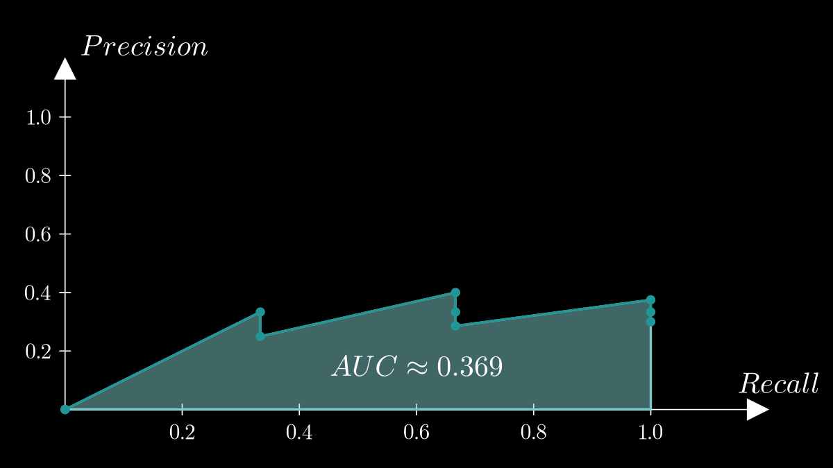
The PR curve is defined by (precision, recall) points, with recall increasing at each relevant item in the retrieved sequence. The PR curve can include additional (precision, recall) points even after recall reaches 1.0, reflecting further retrieved items. However, recall remains constant while precision declines as more non-relevant items are included. This point is discussed in this scikit-learn github issue.
Starting point of PR curve #
In IR textbooks and Victor's lecture, the starting point of PR curve is either (0, 0) or (1/R, 1). However, people often seem to add (0, 1) as the initial point for convention. For example, sklearn does this and precision_recall_curve returns a PR curve including this point (related discussion here). This appears to be another "user-specified" point.
I think it's fine to include this anchor point on Y axis for visualization, as it makes plots look nicer and it's easier to compare different curves this way, but if you need to be mathematically rigorous in IR context I'd avoid including this point. I also found this post mentioning how to plot the first point in the classification context.
Interpolated precision #
This is also commonly known, but in IR evaluation, we often interpolate precision values to smooth out fluctuations (the sawtooth shape) in standard PR curves. This allows for a clearer comparison of PR curves across different systems. However, note that AP does not approximate the area under the PR curve with interpolated precision. 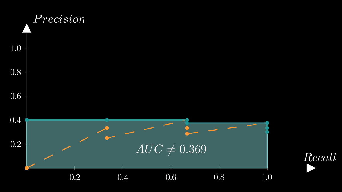
Realistic example #
In the first example, the system was able to retrieve all the relevant items. What if it fails to retrieve all relevant items? Let's imagine another example when the system returns the sequence: $$[1,1,0,1,0,1,0,0,0,0,0,1,0,0]$$ where 1 = relevant, 0 = not, and the number of relevant items is 8. In this case, the recall of PR curve will not reach 1.0 since the system only retrieved 5 relevant items. AP = 0.479 and the PR curve will look like this: 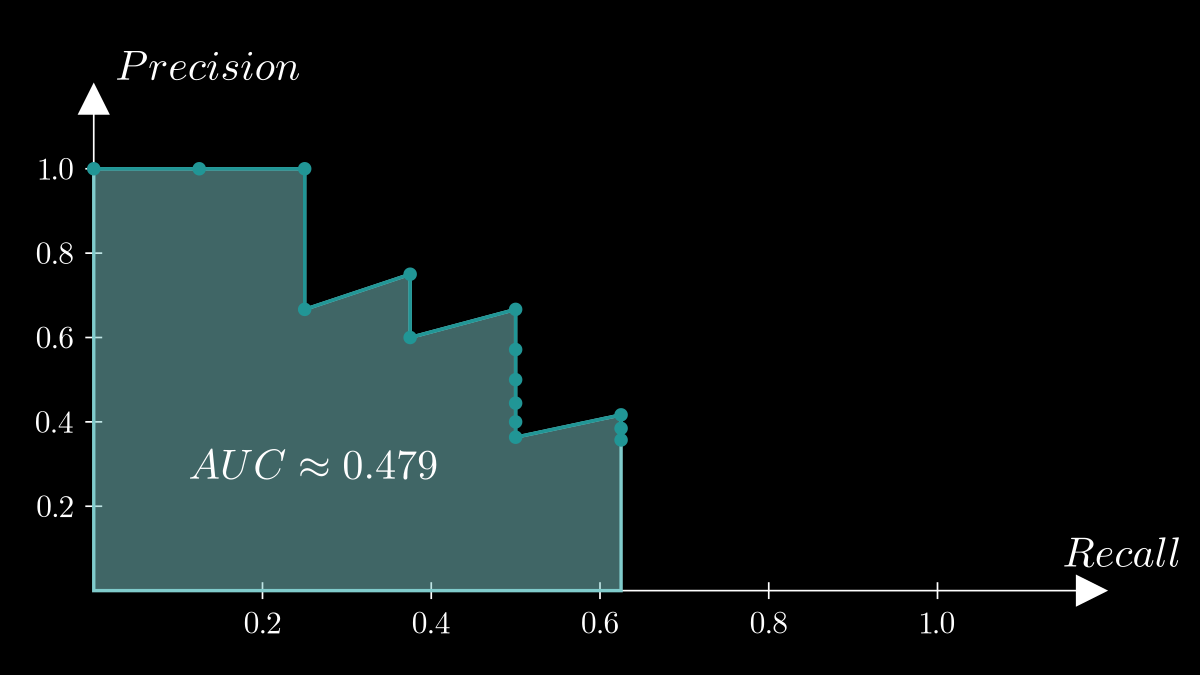
It is normal for the recall of PR curve to not reach 1.0 in the context of retrieval or detection. For classification tasks, the recall of PR curve always reachs 1.0 because the model’s purpose is to classify all given test samples. Most resources don't even mention this, but I found a great Slideshare presentation that clearly explains this in IR context (refer to page 10 and 13). I also found this medium post explaining PR curve in OD context with a practical example where the curve doesn't reach recall=1.0.
Also, notice that we only iterate over the retrieved ranked list to plot the PR curve just like the calculation of AP, rather than going through all the relevant items in the dataset.
Sensitivity to precision #
So far, I've used simple examples where the number of total relevant items is a single digit. To better visualize the PR curve dynamics, let’s scale things up with a case where the sequence length is 1,000 and the number of relevant items is 500 to understand this curve more. We assume that all 500 relevant items were retrieved within this sequence. This is an unrealistic situation in retrieval, but it helps illustrate the intuition behind PR curves when more data points are available.
To see how the distribution of relevant items affects the PR curve, we generate a set of sequences with varying early precisions. Specifically, we incrementally add more relevant items within the first 250 positions across different sequences. To ensure all the curves start from the same point, I fixed the first 10 retrieved items as all "relevant" in every sequence. Here’s the result:
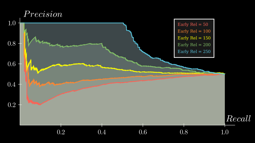
I also highlighted the AUC of curves with a pale color. Notice that the last point of each curve is at (1.0, 0.5) since all sequences have retrieved 250 out of 500 relevant items by the 1,000th item, meaning Precision@1000 = 0.5 at that point. We can observe that the PR curve is very sensitive to the precision of early retrieved items. The more relevant items you miss early on, the sharper the drop in the AP curve corresponding to them.
Here’s another example where we fix the first 50 items instead of 10. The part of the curve that drops to 0.6 remains the same, but it looks like you can still achieve a good AP if you start regaining high precision relatively early.
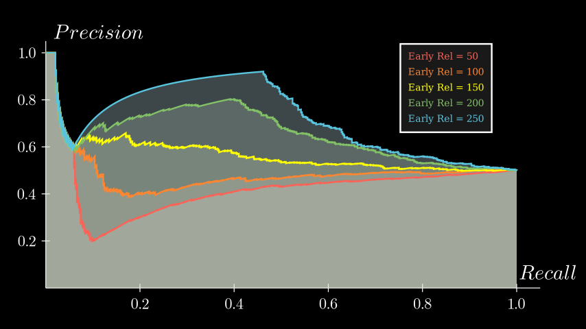
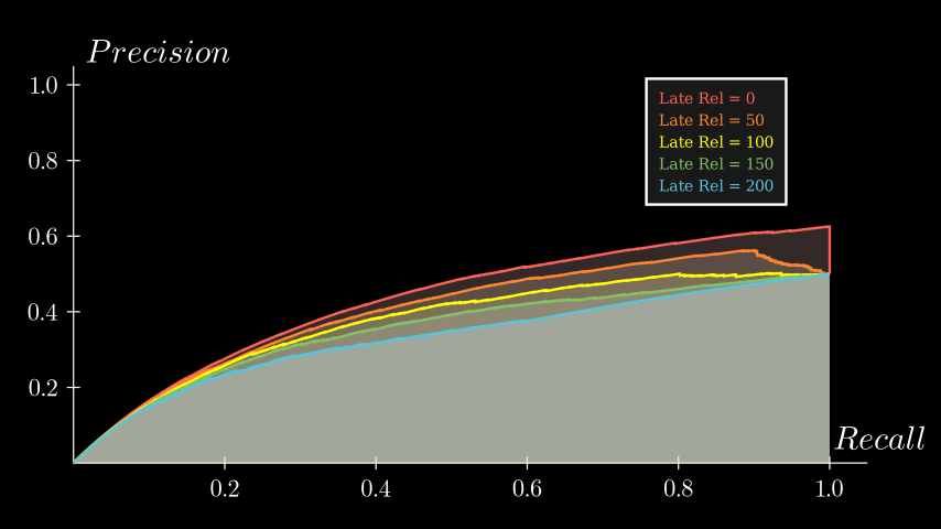
What if you retrieve more the relevant items towards the end? Here's another plot where we vary the number of relevant items retrieved from 0 to 250 in the last 250 items. The remaining relevant items are placed randomly in the rest of the sequence (0~750). In this case, the fewer relevant items you retrieve at the end, the higher the AUC, because that means more relevant items were retrieved earlier.
Relevant items retrieved later in the sequence still contribute to the AUC, but their impact is significantly less compared to relevant items retrieved in higher ranks.
Sensitivity to recall #
Lastly, let’s see how the PR curves change when we vary the number of relevant items retrieved out of 500 actual relevant items. I plotted 5 curves with the number of relevant items in each sequence set to: [100, 200, ..., 500]. Here's the result:
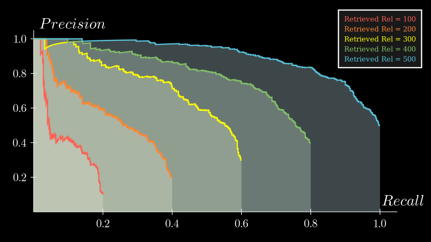
We can see that a higher recall of the retrieved sequence pushes the curves to the right. This makes sense; without relevant items in the retrieved sequence, there are fewer precision values to contribute to the AUC. The more relevant items you retrieve, the more the curve fills out, increasing both recall and the area under the curve.
Historical context #
I also did a bit of research on how this metric became popular among IR researchers, to learn more on why we use mAPs in the first place. I found this lecturenote providing free PDF links for well-known IR books. I explored old IR books with GPT a little bit, and I think it comes down to these 3 reasons:
- Comparing PR curves visually is difficult.
- Single-value overall metric is easier to compare.
- Standardization: AP became a standard metric for evaluating IR systems, especially in early benchmarks like the TREC competitions.
It seems that PR curves were already known and used in evaluation of IR systems in 60s-70s, before the introduction of mAP@K and other averaging metrics. They were pioneered by the works of researchers such as Gerard Salton and C. J. van Rijsbergen.
Salton seems to already recognize issues of PR curve in his earlier works. For example, I found this paragraph in "Introduction to Modern Information Retrieval" third edition, which based on the original Salton's book, which seems to touch the point 1:
Recall-precision graphs, such as that of Fig. 5-2b, have been criticized because a number of parameters are obscured. … Another problem arises when a number of curves such as the one of Fig. 5-2b, each valid for a single query, must be processed to obtain average performance characteristics for many user queries.
Page 159 of the manning's book also mentions point 2:
Examining the entire precision-recall curve is very informative, but there is often a desire to boil this information down to a few numbers, or perhaps even a single number.
From here, evaluation metrics seemed to shift towards "averaging techniques" such as AP@K and "Precision at 11 Recall Levels" (another way to average precisions at fixed recall levels) in 70s-80s. However, it was the TREC (Text REtrieval Conference) in the 90s that particulary accelerated the adoption of this metric.
Before TREC, researchers used different datasets and metrics, making it hard to make fair comparision between IR systems. TREC introduced shared datasets and standard evaluation protocols, similar to what we see in many ML benchmarks today. I think that's why the TREC and metrics used in it became popular from that point on.
My initial misunderstandings #
As someone who is still a noob in IR, whether we're considering the entire database or just the retrieved sequence was the source of my confusion. For example, I wondered why we divide by 3, not the actual total number of relevant items in the earlier example at first, since the definitions of AP available online all say the denominator of AP is "the total number of relevant items". It turns out that I was just looking at the visualization of AP@K while refering to the definition of AP.
At some point, I also misunderstood $N$ in the AP formula as the size of the entire dataset, not the length of the retrieved sequence. but this also turned out to be incorrect as per the definition. AP is defined only for a ranked list of retrieved items. As for the relevant items that weren’t retrieved in the database, we can’t define precisions for those items because they weren’t assigned a rank. This is analogous to the fact that we can't compute precision for non-existent bounding boxes that weren't predicted (it’s obvious when we think of it this way!). However, $N$ can be the size of full dataset if you retrieve the entire dataset by computing a full similarity matrix, for example. Very confusing!
It was also confusing to see how the Precision-Recall (PR) curve in most resources always reaches a recall of 1.0, even though in practice, it's common for the recall of a retrieved sequence to not reach 1.0. After observing PR curves that always reach a recall of 1.0, I mistakenly thought that the definition of AP was normalized locally within the retrieved sequence, using $R_K$ as the denominator.
While this is the case for $AP@K$ in some definitions, it's incorrect for AP because recall is defined based on the total number of relevant items in the dataset $R$, not just the retrieved items. Both AP and the Precision-Recall curve are calculated using the points within the retrieved sequence, but they are normalized by $R$ to account for all relevant items, including those that were not retrieved.
Depending on your prompts, even GPT agents seem to mix these things up. So, I recommend reviewing the official definitions of these metrics in IR textbooks to confirm the standard explanations. For example, page 166 of the Manning's book "An Introduction to Information Retrieval" (PDF link) defines mAP without @K. Another good definition of AP is page 70-71 of the Büttcher et al.'s book (PDF link).
Conclusion #
- AP sums precisions over at all recall levels.
- AP@K only considers the top-$K$ results and has multiple variants depending on the normalization factor.
- AP in IR approximates the AUC of the precision-recall curve.
- mAP in IR is just the average of APs for multiple queries.
Now that I understand mAP, I feel this is a must-have metric for evaluating search systems. It provides a single-value representation of retrieval quality that balances both precision & recall aspects, making it easier to compare different models.
Personally, I’ve decided to adopt $AP@K$ definition with the $\min(K, R)$ term ($AP_2@K$) for evaluation in my projects, as it better accounts for missing relevant items. Hopefully this post gave you a bit more clarity on common IR metrics. Thanks for reading!
References #
Books and papers: #
- Evaluation in Information Retrieval — C.D. Manning, P. Raghavan, H. Schütze (the Manning's book) [PDF chapterlinks]
- Learning to Rank for Information Retrieval — T.-Y. Liu [PDF link]
- Information Retrieval: Implementing and Evaluating Search Engines — C.L.A. Clarke, G. Cormack, S. Büttcher [PDF link]
- Information Retrieval — C.J. van Rijsbergen [PDF link]
- Introduction to Modern Information Retrieval — G. Salton, M.J. McGill, Computer Science Series, 1983 [PDF chapter links] (You need to text search within the page)
- INFORMATION STORAGE AND RETRIEVAL — G. Salton, 1974 [PDF link]
- Inquire: A Natural World Text-to-Image Retrieval Benchmark
Articles & Online Resources: #
- The Smart environment for retrieval system evaluation — G. Salton, 2008 [PDF link]
- The History of Information Retrieval Research
- Performance Evaluation of Information Retrieval Systems
- Mean Average Precision at K (MAP@K) Clearly Explained
- mAP (Mean Average Precision) for Object Detection
- TREC-16 evaluation measuer appendix
- Information Retrieval lecture notes
- Stanford CS 276 / LING 286 Syllabus
- It’s a bird… it’s a plane… it… depends on your classifier’s threshold
- Mean Average Precision (mAP) and other Object Detection Metrics
- Mean Average Precision (MAP) For Recommender Systems